Ames Iowa Housing Prices - Analysis & Regression Model:
Problem Statement:
Which features of a home closely correspond to its price realized at sale? Can we develop a high quality regression model that can predict a home’s sale price after isolating te best quality combinations of features?
Data & Background:
The data for analysis originates from the Ames dataset Kaggle competition for predicting housing prices. The following report discusses the model and results without reference to participation in the competition.
The native dataset was published by the Journal of Statistics Education and includes a Data Dictionary that informed the pre-processing decisions and choices of encoding for categorical features. The original source of the data is information from the county assessor’s office and was compiled by the publisher.
The data includes 78 predictive features that correspond to different attributes of a home in Ames. These features include types that are continuous, discreet, nominal and ordinal. 44 features were categorical with 21 nominal and 23 ordinal respectively. These features were all encoded in advance of modeling.
The feature ‘SalePrice’ is the target for analysis.
A simple linear regression model was used for analysis. Subsequent models were tested using Ridge and Lasso regularization methods. The analysis concludes with the use of Principal Component Analysis (PCA) for feature extraction and comparison of model results.
EDA:
Validating intuition, we can visualize neighborhoods in Ames with the highest average home price:

The feature ‘Year Built’ was also useful for visualization when compared against the sale price. Generally, newer homes fetched higher prices but this background was illuminated further when we set the Seaborn ‘hue’ parameter to different categorical features. Examples are below:
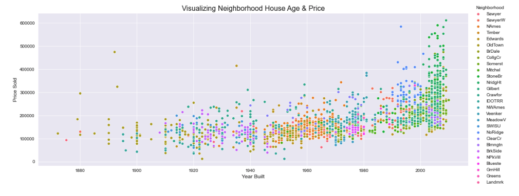
We can see a more precise visualization of neiborhoods that show different average prices when we se the ages of the homes as well.
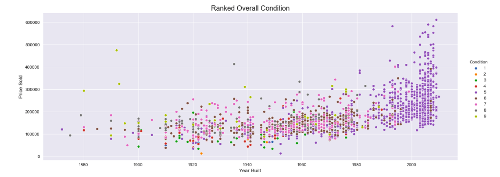
This is an interesting observation that the newest and most expensive homes ranked in the middle for ‘Overall Condition’.
Model Preprocessing:
Most of the preprocessing was to enable encoding of categorical features. All nominal features were One Hor Encoded The ordinal features had their categories standardized to each carry names from best to worst of ‘Ex’, ‘Gd’, ‘TA’, ‘Fa’, ‘Po’ and ‘NA’. Guidance for using these categorical names was taken from the native data dictionary. Standardization was done by mapping dictionaries of the names to each ordinal feature. After standardizing the names, the ordinal features were encoded with Sckit-learn’s OrdinalEncoder method. Ordinally encoded numbers started as ranks from number 5 being ‘best’.
Null values were filled with 0 and irrelevant columns were dropped from the Dataframe.
The total number of predictor features after One Hot Encoding rose to 193 with essentially none of them independent of one another. This became the basis for appling feature extraction with PCA.
Modeling, Regularization & Feature Transformation:
Train Test Split was applied and the data was scaled into z-scores with Scikit-learn’s StandardScaler.
A Linear regression model as instantiated and evaluated before any regularization or PCA. This model was fit with all of the 193 features and delivered dismal results without any regularization or feature extraction. The results of the regression model once regularized are presented below.
R squared is the basis for interpreting model output. We will also consider Root Mean Squared Error (RMSE).
Ridge Model:
Due to the singifant amount of overlapping features, the regularization strength had to be set very high with the Ridge model’s alpha parameter set to 8000.
This regularization strength delivered a training score of .769 and a testing score of .723. This was a significant improvement from when no regularization was applied, with only modest overfitting. Below are the Ridge model metrics:
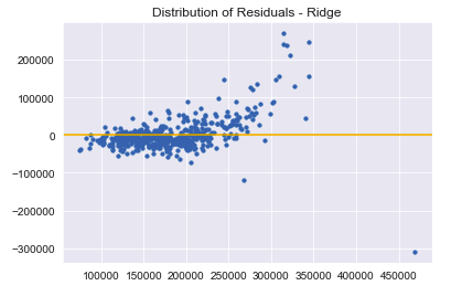
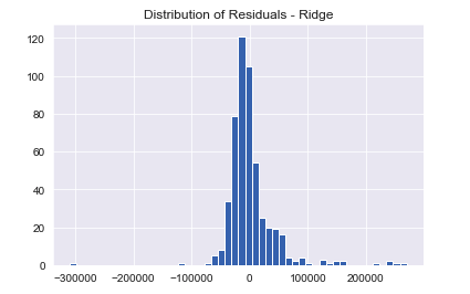
In spite of the decent scores, the Ridge model does not entirely satisfy regression assumptions. The residuals do not quite follow a normal distribution.
The Ridge Model delivered a RMSE of 42,138.50. Transforming this number into dollars we have an idea of the error range of our housing price predictions. This is a high degree of error but it gives us room to experiment further with regularization.
Lasso Model:
The Lasso model also required significantly high regularization strength with a value of alpha at 1500. Alpha having a value this high reduced many feature coefficients to 0 but with only modest improvements to model scores. The Lasso Model printed a train score of .899 and a test score of .757. These scores would only improve minimally even with much larger increases in regularization strength.
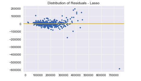
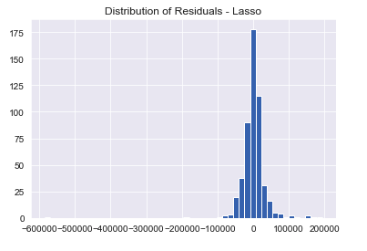
Here and with decent model scores, we can say that the residuals for the Lasso model follow an approximately normal distribution.
The Ridge Model delivered a RMSE of 39,389.44. This is still high but is encouraging for Lasso Regularization in that the model had to analyze the same 193 features with no feature extraction.
We can see now that feature extraction from the set of 193 can likely improve our model’s output and this leads to our next section.
PCA:
The linear regression model was trained on 10 principal components for comparision of output to the previous models. A PCA object was instantiated and fit on the same scaled data.
We can verify that the 10 Principal Components extracted are not correlated with one another in contrast to the 193 previous features:
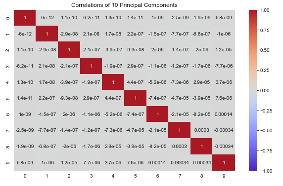
Effectively no correlation to speak of.
The model fit on the 10 principal components delivered a train score of .835 and a test score of .754. This is about the same testing accuracy as the Lasso model but with less overfitting. The PCA model’s metrics are below:
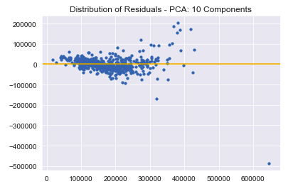

Training the model with PCA also satisfies regression assumptions.
We can also visualize how the principal components individually influence a predicted sale price by charting the values of each component’s coefficient:
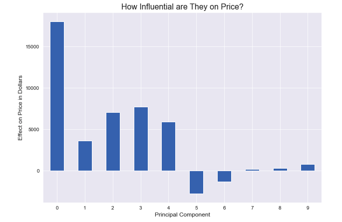
Fascinating result showing the marginal decrease in influence with each new Principal Component.
The RMSE for the PCA model was 39,623.19. This is slighly higher than that of the Lasso model but again with less overfitting. Further experiments with different hyperparameters for PCA can be done to see if this metric can be improved.
Conclusions & Next Steps:
The models’ predictions were respectable. The RMSE scores were high, but were reduced in a pattern that points to the appropriateness of using regularization and feature extraction for improiving model results.
Lasso regularization and PCA offered two directions for managing the initially large and unmanageable amount of features. Starting with different subsets of these features or using more advanced modeling techinques can be another point of departure on what was discovered from the models.
Additional experiments with different numbers of Principal components can also be conducted to see if PCA is a relaible improvement with respect to Lasso regularization.